A New Coordinate System
In the xy-plane — called a Cartesian Coordinate System — imagine a point with coordinates (3, 2). Decrypting this mathematical code means that there is a point located in the area where the lines x = 3 and y = 2 intersect. Imagine x = 3 as a scaling of x = 1, 3 times. In other words, we can always write respective positions of points in terms of x = 1 and y = 1 by just counting how many times that distance from x = 0 to x = 1 has to be multiplied to get to the x-position the point is located at. Let’s do the same for y as well, to establish strict geometrical definitions for what it means to be located in our coordinate plane.
Now imagine this same point, but now we draw a line connecting the point to the origin, and make the tip of this line (the area where the point originally was) an arrow, to indicate the direction it’s going.
This is a new mathematical object and therefore let’s use brackets [ ] to replace the parentheses, and instead of writing [3, 2] horizontally, let’s write it vertically:
v = [ 3, 2 ]
Note: Whenever you see brackets [a, b], just know that the numbers inside are positioned so that "a" is placed above "b".
Now recall that the location of these points are based on some fixed distance from the origin. Because this distance is going to be consistently one, let’s call it a unit distance — unit means 1 — so for our new mathematical objects, let's create fixed unit distances to be able to accurately describe this line going in a direction, by locating the end point.
This pointy line, we’ll call a vector, instead of a point. Then while we’re naming things, let’s call that fixed distance from the origin along the x-axis, “i-hat”. Then that fixed distance along the y-axis, “j-hat”. The geometrical essence of doing this allows us to describe any vector in our coordinate system in terms of these “basis vectors” i-hat and j-hat. Essentially, we can describe what the entire coordinate plane — which is composed of every possible vector — does by just tracking these basis vectors as they change, or transform.
“Abstract” Vector Space
All of these vectors and this coordinate plane all exist, right? Depends — they are called “abstract” objects because they really only live conceptually in our minds as a logical tool we use to solve some problems. Every mathematical object is abstract.
For example, you can’t point to the number 3. Any number is an abstract concept which implies it has some sort of generality to it. If I say 3, it could mean a list of things; it’s “generalized”.
Our vectors are also an abstract tool, and we can do a list of things with them; they’re all generalized under the idea of “Linear Transformations”.
Isn’t Linearity Like Being a Line?
Linearity, in linear algebra, provides the fundamental “axioms”. Everything in math works under some assumptions, some foundational thoughts, that we all hold to be true. These are called “axioms”.
2 + 2 can only equal 4 if addition is the counting of successor terms in a sequence, and 4 is the second successor to 2. These are obvious when we think about math in a practical sense — like I have 2 jars and then I’m given 2 more, so now I have 4.
The only issue with this is that at a high level, more pure math (less correlation to practical application, currently) uses addition a little differently, as we will see with vector operations, and computing determinants.
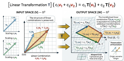
In a geometric sense, the formal rules of linearity state that all vectors in our vector space can only be changed in a restricted manner so that their transformed version can be expressed as adding and scaling the original vector. Only when this requirement is met, can a transformation be understood as a linear transformation.
That explanation is kind of vague, like what transformation wouldn’t be linear?
Well, an enforcing idea you can think about is the fact the grid lines on our coordinate plane should stay parallel to each other and evenly spaced. The space between them can change — which is really important for the determinant — but it can’t be uneven. Additionally, the origin has to stay fixed in place, otherwise asymmetry shows up which is bad.
Linearity gets its name from a foundational symmetry-preserving behavior of everything which is deemed “linear”. This preservation of geometric symmetry is what allows us to be able to mathematically describe each action we make, only if it’s symmetrical.
In theory, if you're curious, a nonlinear transformation is also able to be described mathematically (in a field like complex analysis with the Riemann Zeta function) but is fundamentally more complicated than this class of linear transformations.
Vectors vs. Points
Points just tell you the location of one little spot in the coordinate plane, with an x and y coordinate: two bits of information.
Likewise, vectors have a given length (distance from the origin) which is referred to as its “magnitude”, and a “direction” which is where the arrow is pointing. Therefore we have two different bits of information. We are representing the same point with two different numbers. Vectors use magnitude/radius and direction/angle, so they’re graphed like they’re on the polar coordinate plane. Points use horizontal and vertical axes, so they’re graphed on the Cartesian coordinate plane.
Vectors tell us a lot more about linear transformations. For example, let’s say a transformation rotates the basis vectors by 90° counter-clockwise. This tells us that every vector will have to point in a direction 90° counter-clockwise from where it originally was pointing, therefore we can prove that the entire vector space… rotates 90° counter-clockwise.
Changing Space
Imagine you’re playing around with this coordinate plane we’ve designed and you’re performing different linear transformations. You’ll realize every linear transformation other than two actions — rotation, and doing nothing (referred to as the identity matrix) — stretches space in some way. This is an important characteristic of what our vectors are doing. Let's mathematically describe this scaling of our coordinate plane by looking at the Unit Square.
The unit square has side lengths of i-hat and j-hat.
i-hat is 1 unit distance away from the origin horizontally,
and j-hat is 1 unit distance away vertically.
Area = 1 * 1 = 1
By measuring how the area of this unit square changes by some multiplier as a result of a linear transformation (due to the laws of linearity, the unit square cannot be stretched asymmetrically, making calculating the area very easy):
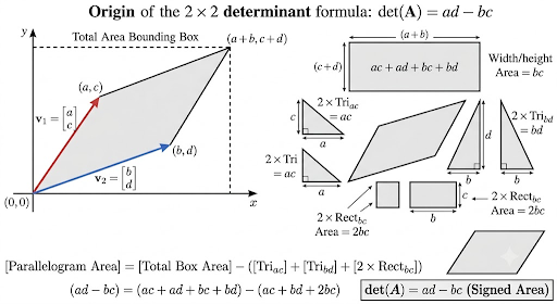
This number that we’re measuring is called the determinant of the linear transformation. It’s called that because it determines the effects that the linear transformation enacted on the vector coordinate plane.
Measuring the Determinant
To start, let’s represent linear transformations mathematically.
Any linear transformation can be represented by the position of the column vectors after the transformation. Recall earlier we represent 2D vectors as [a, b].
i-hat = [ 1 0 ], j-hat = [ 0 1 ]
Combining these two vectors together we get a matrix:
Identity Matrix = [ 1 0, 0 1 ]
This is called the Identity Matrix and it represents our coordinate plane in its standard position.
Assume a linear transformation produces the matrix [ 3 0, 0 3 ]. This means i-hat is now located at (3, 0) and j-hat at (0, 3). The transformation scaled our coordinate plane by a factor of 3, so therefore the determinant of this matrix is 3.
A general formula can then be derived for a 2 * 2 matrix (which means a linear transformation affecting i-hat and j-hat in two dimensions) using geometry to find the area of the transformed unit square defined by i-hat and j-hat.
Higher Dimensional Space
As explained prior, observing more abstract mathematical dimensions means looking at more axes. For the third dimension we include the z-axis, with the basis vector known as k-hat.
With each new dimension that we want to observe in the vector space, we represent that in mathematical notation by adding a new row to our matrix.
In short, more rows means more dimensions. We can have a matrix where we measure i-hat (first dimension basis vector) and j-hat (second dimension basis vector) in ten dimensions (referred to as a 2 * 10 matrix), but the 8 entries after the second dimension are always going to be 0 unless we perform matrix multiplication.
Matrices in Math Problems
The most common matrix multiplication you often see computationally is Matrix-Vector Multiplication:
v' = A * v
In short, you’re looking at the initial vector (which is usually on the right) and performing the linear transformation encoded by the matrix on the left of it. In traditional math equations, there's a section on the left and a section on the right of the equals sign.
We read each section left to right for order in traditional equations.
In equations involving matrices, it’s easier to read the sections from right to left.
This is because when looking at transformations acting on our initial vector (always on the right), we perform the linear transformation which is directly attached to the initial vector first, and then the next linear transformation:
v' = B * A * x
where B and A are matrices encoding linear transformations, and A is always performed first.
Matrix-Matrix Multiplication is literally what I described above — performing a sequence of linear transformations in a specific order.
It’s important to know that the commutative property of multiplication does not apply in matrix operations (A * B != B * A). This is a fact which can be realized when pondering about how they’re defined and experimenting with linear transformations.
Note: This page covers fundamental geometric concepts for basic linear algebra. Additional sections on matrix inversion, eigenvectors, and eigenvalues will be added in future updates.
![Standard Unit Square (i, j) diagram showing basis vectors i = [1,0] and j = [0,1] and area 1](images/linear-algebra-2.png)